The environmental changes of glacial periods greatly influenced the evolution and present-day distribution of terrestrial and aquatic species. Most populations persisted in glacial refugia -ice-free areas from which they began to colonise northern regions as environmental conditions improved during post-glacial periods. In addition to influencing species distribution, these climatic changes shaped species ecology, in some cases leading to shifts in diet, habitat, and behaviour. While these patterns have been extensively studied for terrestrial species during the last glacial period (26.5 – 19 kya), the same is not true for aquatic ecosystems. Yet thousands of fossils of fish, particularly salmonids, have been found at numerous Palaeolithic archaeological sites across Europe.

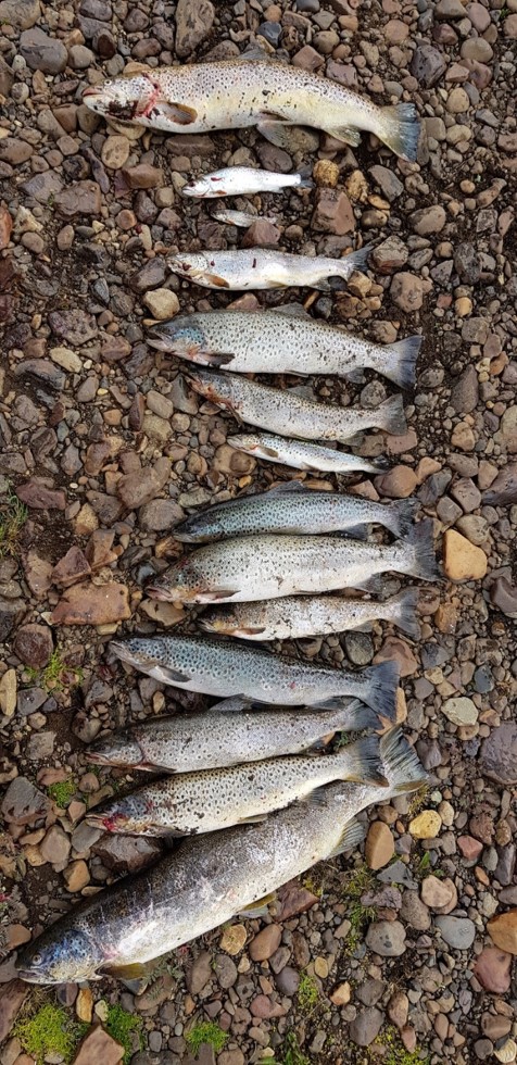
Understanding how the last glacial period impacted the phenotypic diversity of brown trout (Salmo trutta Linnaeus 1758), a species of salmonid with vast phenotypic diversity and adaptive capacity, might provide insights into fish ecology and evolution, the impact of past climate changes on intraspecific biodiversity, and human reliance on fish resources in the past. Brown trout is a facultative anadromous species, which means that individuals with very different life cycles co-exist within the same population: some migrate to the sea (or estuary, lake) during maturation (migratory individuals, aka anadromous if they migrate at sea) and then return to the river for reproduction, while others remain and grow in freshwater (resident brown trout). These two different strategies involve phenotypic changes in colour, diet and size and have consequences for survival. For example, while migration entails risks for the survival of the individual, it increases reproductive success (a higher growth rate can lead to greater fertility, especially in females). Resident trout growth rates are usually lower, but survival is less at risk. The presence of both strategies is advantageous for the survival of the species, which can thus exploit different environments and colonise new habitats through migration. Studying this aspect of brown trout is therefore crucial in an exceptional context such as the ice age. Together with migratory status, growth rate is another noteworthy phenotypic feature, correlated to the individual’s health, migratory status and fertility. The growth rate of brown trout strongly depends on temperature, which thus also modulates the age at migration. During the ice sheet maximum extension between 26 and 19 kyr B.P., lower temperatures might have determined reduced growth rates in brown trout and, in general, lower productivity in the ecosystem.

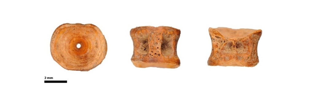
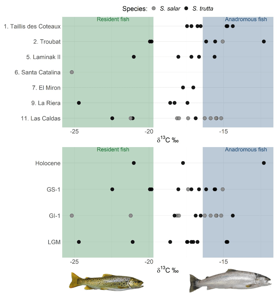
To reconstruct these aspects of the phenotypic diversity of S. trutta, we studied brown trout archaeological vertebrae dating back to approximately 30–9 kya, found in the northern part of the Iberian glacial refuge (northern Spain and France up to the Loire). This sampling allowed the study of phenotypic variation over time (pre-, during, and post-LGM) and space (the core of the refugium, Spain, and north of the refugium, France). The inference of migratory status using the stable isotope carbon-13 (which has differential values in marine and freshwater environments) showed a continuum of migratory strategies throughout the studied period. Together with migratory individuals displaying a classic anadromous life cycle and resident individuals, several fish with intermediate signatures were found. We interpreted these as fish that either spent a variable period in freshwater before and/or after sea migration, behaviour also observed today, or migrated to low-salinity regions, such as estuaries or the English Channel during post-LGM.

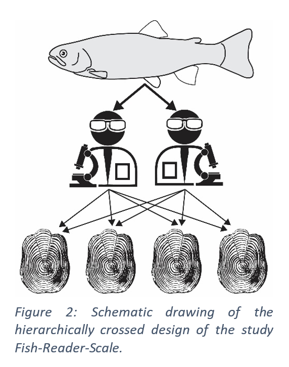
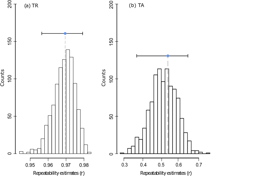
Age, body length, and average growth rates, calculated through vertebrae size and sclerochronology, fell within the range observed for contemporary brown trout populations.

Overall, the results demonstrated brown trout acclimation to the climate changes of the last glacial maximum, confirming the adaptation capacity of the species to low temperatures and the role of Iberia in maintaining its diversity. Moreover, the persistence of the migration capacity implies that these populations could have potentially colonised the northern regions of Europe after deglaciation.

As a last thing, this study suggests that the inland regions of France were more affected by the shift in the climatic conditions as brown trout showed significantly lower growth rates in this region during the LGM and no resident brown trout was found in the northernmost archaeological site in France (Taillis Des Coteaux), possibly indicating harsh local conditions pushing the individuals to migrate to sea, which is usually less sensitive to climatic changes than river habitats.

Take-home message: The phenotypic diversity of brown trout during the last glacial maximum in the Iberian glacial refugium was maintained and comparable to the current one.

References

Ambra D’Aurelio, Lucía Agudo Pérez, Lawrence G. Straus, Manuel R. González Morales, Arturo Morales-Muñiz, Jerome Primault, Jean-Marc Roussel, Laurence Tissot, Stephane Glise, Frederic Lange, Camille Riquier, Michel Barbaza, Eduardo Berganza, José Luis Arribas, Pablo Arias, Aurélien Simonet, Ana B. Marín-Arroyo, Joelle Chat, Françoise Daverat (2025). Phenotypic diversity of brown trout (Salmo trutta L.) during the late Upper Pleistocene and Early Holocene in the glacial refugium of Iberia,
Palaeogeography, Palaeoclimatology, Palaeoecology, Volume 675, https://doi.org/10.1016/j.palaeo.2025.113073

Clark, P. U., Dyke, A. S., Shakun, J. D., Carlson, A. E., Clark, J., Wohlarth, B., Mitrovica, J. X., Hostetler, S. W., & McCabe, A. M. (2009). The Last Glacial Maximum. Science, 710–714.

Ferguson, A., Reed, T. E., Cross, T. F., McGinnity, P., & Prodöhl, P. A. (2019). Anadromy, potamodromy and residency in brown trout Salmo trutta: The role of genes and the environment. Journal of Fish Biology, 95(3), 692–718. https://doi.org/10.1111/jfb.14005

Hewitt, G. (2000). The genetic legacy of the Quaternary ice ages. Nature, 405(6789), 907–913. https://doi.org/10.1038/35016000

Ménot, G., Bard, E., Rostek, F., Weijers, J. W. H., Hopmans, E. C., Schouten, S., & Damsté, J. S. S. (2006). Early Reactivation of European Rivers During the Last Deglaciation. Science, 313(5793), 1623–1625. https://doi.org/10.1126/science.1130511

Nevoux, M., Finstad, B., Davidsen, J. G., Finlay, R., Josset, Q., Poole, R., Höjesjö, J., Aarestrup, K., Persson, L., Tolvanen, O., & Jonsson, B. (2019). Environmental influences on life history strategies in partially anadromous brown trout (Salmo trutta, Salmonidae). Fish and Fisheries, 20(6), 1051–1082. https://doi.org/10.1111/faf.12396

Brown trout (Salmo trutta) is a highly sought game species, while also considered as patrimonial in many countries and regions over its whole distribution area, Eurasia. It is also a species, consequently, that has a strong interaction with humans : through fishing over many millennia, but also through translocation, and very intensive stocking since 150 years. Meanwhile, geneticists have shown that the species harbours wondrous levels of genetic diversity that have been shaped over hundred of thousands years. Five distinct lineages have at least been identified, among which the Atlantic (ATL) and Mediterranean (MED) lineages, occupying roughly the Atlantic side and Mediterranean side of Europa, roughly.

Pictures of brown trout originating from two different lineages. The Atlantic lineage (ATL) is characterized by large spots (orange arrow) and the presence of a visible lateral line (green arrow). The Mediterranean lineage (MED) displays a very large quantity of small black spots, a few vertical black stripes (black arrows), but no visible lateral line.

Worldwide efforts of introduction or restocking in the initial distribution area however was done mostly using the ATL lineage. The most striking consequence was the massive creation of hybrids and the introgression of ATL genes into local native lineages, well described by geneticists. Biodiversity managers have consequently attempted different strategies to protect the MED lineage, and possibly remove ATL genes. One such strategy that was partially successful is the translocation of native MED fish into areas where ATL genes are dominant. Partially only, because, if the proportion of ATL genes declined, the proportion of hybrids (HYB) increased.

Picture of a hybrid brown trout. The vertical stripes are roughly visible as in a MED trout, but the number of spots relates more to an ATL trout.

More recently however, we uncovered behavioural and selective mechanisms involved in the fitness of hybrids. More specifically, it appears that offspring of MED females survive much better in cold waters than those of ATL females: this is evidence for a temperature based genotype / environment interaction. And temperature fluctuates temporally, but also spatially. Could such an eco-evolutionary mechanism be involved significantly in the maintenance of hybrid genotypes ?

The relation between offspring, survival, temperature and maternal introgression. Offspring from MED females fare better in cold waters.

To answer this question, we built a simulation demogenetic model, wherein we replicated the actions of the biodiversity managers, accounting (or not) for the genotype / environment described above. Basically, we simulated the translocation of MED individuals from the downstream part of a river to the upstream part, previously stocked with ATL fish.

Simulation scenario, based on the actual translocation protocol : in 2005, a rather large number of MED fish was caught downstream and released in the upstream area, where only ATL fish were present. The biodiversity managers then tracked introgression for several years afterwards.

The model proposed two trajectories, depending on the inclusion of the genotype / environment interaction. Without this interaction (neutral scenario), introgression in the upstream area barely declined. But with the interaction, the introgression declined quickly in 2 generations. Yet meanwhile, a very large number of hybrids were created.

The cool thing is, the neutral scenario was very far from reality (introgression data provided by biodiversity managers), whereas the genotype / environment scenario was much closer, indicating that this eco-evolutionary mechanism is rather likely to be responsible for a large part of the observed dynamics of introgression.

Take-home message : eco-evolution is clearly interacting with our management practices, possibly on very short time scales, and with massive effects.

References of interest :

Dorinda Folio, Arnaud Caudron, Laure Vigier, Sylvie Oddou-Muratorio, Jacques Labonne. Using eco‐evolutionary models to improve management of introgression in brown trout. Ecology of Freshwater Fish, 2024, ⟨10.1111/eff.12789⟩. ⟨hal-04603141⟩

Dorinda Folio, Jordi Gil, Arnaud Caudron, Jacques Labonne. Genotype‐by‐environment interactions drive the maintenance of genetic variation in a Salmo trutta L. hybrid zone. Evolutionary Applications, 2021, 14, pp.2698-2711. ⟨10.1111/eva.13307⟩. ⟨hal-03420466⟩

Jordi Gil, Jacques Labonne, A. Caudron. Evaluation of strategies to conserve and restore intraspecific biodiversity of brown trout: outcomes from genetic monitoring in the French Alps. Reviews in Fish Biology and Fisheries, 2016, 26 (1), pp.1-11. ⟨10.1007/s11160-015-9405-y⟩. ⟨hal-01901371⟩

Amaia Lamarins, Victor Fririon, Dorinda Marie Folio, Camille Vernier, Léa Daupagne, et al.. Importance of interindividual interactions in eco‐evolutionary population dynamics: The rise of demo‐genetic agent‐based models. Evolutionary Applications, 2022, 15 (12), pp.1988-2001. ⟨10.1111/eva.13508⟩. ⟨hal-03909303⟩

Every biologist needs a book to read in the life of its favoured organism. For ichthyologists, teleost scales have been telling stories over a century. Because of their external position, they are easy to remove. Among other applications, they give access to life history traits, such as age (at maturity or at migration) and growth (Figure 1). By delineating annuli (yearly rings deposited during winter) and measuring the associated interannuli spacing, one can estimate an individual’s growth trajectory and migratory status (Elliott and Chambers, 1996); however, measurements may vary across readers and scales, for a same fish.

Figure 1: Scale of a sea trout reflecting its life history traits.

Over time, researcher have come to the acceptance that multiple readings (numerous scales or numerous readers) are better to gain reliable information (Panfili et al., 2002). However, the number of scales or readers required to determine life history traits is not that easy to define because first, it depends on the fish species and second, the mention of the required methodology for one species is rarely explicit in the literature.  Over the past 30 years, the number of validation studies has increased (Campana, 2001), yet the number of required readings to capture biological variability is still unclear. When is it required to proceed to multiple readings? Which variable needs multiple readings (age, growth)? Should we read several scales, or have several readers, or both ?

Individual variation has become a foremost concern in biology, it is therefore paramount to come up with sampling designs able to minimize sampling effort while keeping information level steady: indeed, a reasonable shortcut to avoid redundancy and a waste of resources. Following that idea, Lucie Aulus and colleagues sampled scales of 60 fish originating from the Kerguelen Is. (one of our beloved destinations). For each fish, they determined total age at capture by counting annuli (TA) and measured the total radius (TR) on 4 different scales, using two different readers in a double blind manner (Figure 2).

They then decomposed data variance hierarchically in a nested and crossed manner, namely Fish–Reader–Scale to determine which levels account for the variance in growth and age (Figure 2). The reliability of both scale total radius and fish age was estimated by the r repeatability coefficient (Stoffel et al., 2017). This coefficient ranges from 0 to 1, a high value indicating that a similar result is more likely to be observed when repeating the observation (or measure) under consistent conditions.

Figure 3: Repeatability estimates (r) of (a) total radius (TR) and (b) total age (TA). Symbols and dashed lines indicate the median of the repeatability estimates (r) of Fish level, with uncertainty (i.e. 95% confidence intervals) indicated, obtained over 1000 bootstraps.

For scale total radius (TR), the repeatability was extremely high (97%, Figure. 3a), meaning that whatever the reader or the scale, the measure of total radius was very stable. Basically, it means that when sampled in a relatively well located area on the fish, total radius would be well estimated by using a single measure on a single scale by a single reader. On the contrary, for total age (TA) the repeatability was about 53% (Fig. 3b). Readers indeed sometimes disagreed in delineating annuli on a same scale, or different scales from a same fish provided different age readings consistent between readers.

So, two variables, but not the same repeatability, and yet, these two variables are often associated in various analyses, for instance, to build growth models. The present case study thus indicates that if age is a relative problem, total radius is not, and therefore total radius might not need to be sampled on every scale samples (avoid redundancy, right?). Second, by estimating repeatability, we also estimate the different sources of errors: these error estimates can be later reinjected into further models for total age, wherein we would read less scales per fish, allowing us to increase the number of fish studied for the same effort (to prevent wasting resource).

As soon as one envisions important amounts of scale analysis, such preliminary investigations to quantify errors should be a prerequisite: it can provide valuable insights for accurate modelling of individual variability. Such understanding of interindividual variability could have several applications in stock assessment and conservation. It could also save significant amount of resources for retrospective studies, for which scales collections are invaluable assets.

More details on our study here:

Aulus-Giacosa L., Aymes J.-C., Gaudin P., Vignon M. (2019) Hierarchical variance decomposition of fish scale growth and age to investigate the relative contributions of readers and scales. Marine and Freshwater Research , -.

Cited literature:

Campana, S.E., 2001. Accuracy, precision and quality control in age determination, including a review of the use and abuse of age validation methods. J. Fish Biol. 59, 197–242. https://doi.org/10.1111/j.1095-8649.2001.tb00127.x

Elliott, J., Chambers, S., 1996. A guide to the interpretation of sea trout scales., R & D Report. National Rivers Authority, Bristol (UK).

Panfili, J., De Pontual, H., Troadec, H., Wright, P.-J., 2002. Manuel de sclérochronologie des poissons, Editions Quae. ed. IFREMER : IRD, Plouzané, Paris ; France.

Stoffel, M.A., Nakagawa, S., Schielzeth, H., 2017. rptR: repeatability estimation and variance decomposition by generalized linear mixed-effects models. Methods Ecol. Evol. 8, 1639–1644. https://doi.org/10.1111/2041-210X.12797

Semelparous animals breed once, then die. But what does “once” mean? Some species comply with the so-called big bang reproduction, such as the well named Ephemera (mayflies), which lay one clutch of eggs and die within the same night. However, many species are considered semelparous while breeding several times within a single breeding season. Semélê herself mated several times with Zeus before being thunderstruck, admittedly after (in fact before) giving birth for the first time. Allis shad is such a semelparous species. It is also a capital breeder with determinate fecundity, which means that these fish start their one-month long spawning season with finite stocks of energy and eggs. They face an optimization challenge: matching egg and energy exhaustion. It would not be adaptive for them to either squander their energy and die with unlaid eggs, or survive long after having laid their last eggs. This challenge exists for every living organism, but it is probably more meaningful to species like Allis shad, which face a particularly steep rate of energy and egg exhaustion until death.

With this in mind, we documented the schedule of spawning acts and energy consumption of a few Allis shad in the field. For this, we caught them at the Uxondoa dam on the Nivelle River (Basque Country), at the end of their upstream migration, and tagged them with accelerometers that logged data (3D acceleration + temperature + pressure) until the fish’s death. Four kinds of information were obtained from these data (Fig. 1).

Fig. 1a

Fig. 1b

Fig. 1c

Fig. 1d

Figure 1. (a) shad spawning and (b) the corresponding 3D acceleration (xyz: red, green, blue) and pressure (pink) signal. (c) Tail beats and the corrsponding wave on the z-axis. (d) Tag verticality as an indicator of fish’s roundness.

First, as the spawning act consists in the fish pair spinning for a few seconds in approximately five one-meter diameter circles while thrashing the water surface with their tail, the corresponding pattern of acceleration and hydrostatic pressure was detected to assess the number and timing of spawning acts. Second, average tail beat frequency and temperature were computed for every minute and transformed in energy expenditure, using a model built for American shad^1,2. Third, the gravitational component of acceleration was used to regularly compute the angle between the tag and the vertical, an indicator of fish’s roundness. Fourth, the exact timing of death was detected as both a null dynamic acceleration indicating immobility, and a shift in gravitational acceleration indicating the fish rolled on its flank. Dead fish were retrieved, in order to collect the accelerometers and their data, and weigh the fish and their remaining oocytes.

Figure 2. The schedule of spawning and energy consumption. (a) Timing of shad spawning acts in the season – each colour is a different individual. (b) Cumulated energy consumed, estimated from temperature and tail beat frequency. (c) Change in tag verticality.

On average, a shad female performed 16 spawning acts distributed in six nights each separated by four nights without spawning (Fig. 2). The timing of spawning seemed to be influenced by both the physical and social environment, since the probability of spawning during one night increased with temperature, and spawning acts within a night were temporally aggregated both intra- and inter-individually. The metabolic model fed with temperature and tail beat frequency predicted a very steep energy consumption: on average 0.19kJ.min^-1, summing to 7193kJ for 26 days of spawning activity, more than American shad during their 230km and seven-week long upstream migration in the Connecticut River². Accordingly, shad thinned rapidly, especially during nights, and lost up to 53% of their initial weight. They died on average four days after their last spawning act, retaining 80g of ovaries, while the initial weight must have been around 200g.

So, shad females seem to rapidly expend their energy while spawning, and die with a significant amount of remaining eggs. Yet, shad in the Nivelle only have to ascend 13km to reach spawning grounds. How would they manage their spawning energy after a long upstream migration in a dammed river, with warming water? This management of egg and energy stock might be crucial for population conservation³. Methodologically, this study is a further step towards the monitoring of spawning activity and related energy expenditure in the field, and the field is where we (at least some of us) like to be!

Read the full story on BioRXiv: https://doi.org/10.1101/436295

Cited literature:

Density-dependence is a fundamental principle in ecology: it states that the growth, the survival, the fitness of individuals is directly related to local density. This is so because trophic resources are limited, a point stated by Malthus in 1798 that inspired Darwin’s theory of natural selection. Malthus had indeed predicted that demographic parameters should change with density. One interesting consequence of density dependence is that it tends to promote homeostatic dynamics: when density is low, survival is increased so to reach quickly an equilibrium point; once reached, the population size will not increase greatly simply because survival decreases due to high density. In a nutshell, this is the concept of population “resilience”.

Fishes, and especially salmonids, are no exception to this natural law. When resources per capita change, then individual fitness changes accordingly. Of course, if resources, or access to resources, are controlled by environmental variation, then environmental variation controls density dependent mechanisms in salmonid populations. There is a wealth of papers describing this density dependence in natural or experimental environments.

Ranking among one of the most potent environmental change, rainfall variation shapes many aspects of salmon life history. It controls for trophic resources by affecting the availability of preys, but it also determines local density for salmon themselves, by changing water discharge in rivers. Climate change reshuffling our knowledge of rainfall patterns, it becomes paramount to investigate how this parameter can affect the resilience of salmon populations.

Our lab set up an experiment in a semi-natural channel, where we introduced wild Atlantic salmon juveniles from known parents. In this channel, we created several replicates for a simple design combining two density levels (2.5 and 5 fish.m²) and two water discharge levels (Low Flow =70 m³.h^-1 and High Flow = 110 m³.h^-1, see Figure 2). 4 replicates were created for each condition, totalizing 960 juveniles originating from 7 families. We monitored individual growth and survival in each experimental condition especially during the first summer. The data indicate that at High Flow, survival and growth are strongly controlled by density: this was the expected mechanism at work, which fosters population resilience. But at Low Flow, this density dependent effect nearly disappeared, on both survival and growth. Environmental change, through river flow dynamics in summer, would impact negatively one of the fundamental mechanisms that govern the persistence and stability of salmon populations.

Although this pattern itself is already interesting, because it teaches us that the dynamics of our resources may be less resilient than it used to be, it also shadows a number of possible explanations that are probably not mutually exclusive. You can discover more about this experiment: family effects, standard metabolism, and expression of nutritional metabolism related genes, it is all here.

References:

Bardonnet A., Lepais O., 2015. Interactions and effects of density, environment and parental origin on Y-O-Y Atlantic salmon survival, growth and early maturation. IV International symposium on « Advances in the population ecology of stream salmonids”, May 25-29, Girona, Spain.

Bardonnet A., Lepais O., Bolliet V., Panserat S., Salvado J.-C., Prévost, E., 2017. Impact of low flow on young-of-year Atlantic salmon: density-dependent and density-independent factors interact to decrease population resilience. 50th Anniversary Symposium of the Fisheries Society of the British Isles, 3-7 July, Exeter, UK.

References

Applegate, V.C., 1950. Natural history of the sea lamprey, Petromyzon marinus, in Michigan (Federal Government Series No. 55), Special Scientific Report – Fisheries. U.S. Fish and Wildlife Service, Ann Arbor, Michigan: University of Michigan Library.
ECP, 2018. Ecology and Fish Population Biology Facility. https://doi.org/10.15454/1.5572402068944548E12
Gracia, S., Caut, I., Carry, L., 2016. Suivi de la lamproie marine sur la Dordogne et la Garonne. MIGADO.
Kery, M., Schaub, M., 2011. Bayesian Population Analysis using WinBUGS: A Hierarchical Perspective. Academic Press.
Kynard, B., Horgan, M., 2019. Long-term studies on restoration of Connecticut River anadromous sea lamprey, Petromyzon marinus Linnaeus 1758: Trend in annual adult runs, abundance cycle, and nesting. Journal of Applied Ichthyology 35, 1154–1163. https://doi.org/10.1111/jai.13967
Manion, P.J., Hanson, L.H., 1980. Spawning Behavior and Fecundity of Lampreys from the Upper Three Great Lakes. Can. J. Fish. Aquat. Sci. 37, 1635–1640. https://doi.org/10.1139/f80-211
Migradour, 2010. Suivi de la reproduction de la Lamproie marine sur le bassin de l’Adour – Tranche 1/3, gaves et nives.
Royle, J. andrew, Dorazio, R., 2012. Parameter-expanded data augmentation for Bayesian analysis of capture-recapture models. Journal of Ornithology 152, 521–537. https://doi.org/10.1007/s10336-010-0619-4
I’m picky.
Observations of reproductive behaviors in sexually reproducing organisms indicate that many species can be “choosy”: they tend to be selective for their partners quality. Mate choice has costs and potential benefits that are likely to vary depending on individual characteristics (e.g. sex, quality), and on social context (number of potential partners). And if you are too picky, that cost may have dire consequences: you will end up alone.
The dilemma of finding a mate in a fluctuating world, and the outcomes of being more or less choosy. It is a very old question, since sex appeared more than a billion years ago on Earth. Considering however the amount of internet bandwidth devoted to dating interactions, it will probably remain a central matter for centuries to come.
Classically, scientific literature predicts that the limiting sex (in term of gametes) – females – should be choosy, whereas the common sex – males – less so or not at all, or in very peculiar situations. Indeed, as a result of anisogamy (unbalance between gametes number and/or size between sexes), female’s reproductive rate is lower than males, making ready to mate males more numerous than ready to mate females and thus generating stronger mating competition among males. But who is really ready to mate, with which partner with regard to quality, and for how long? This is what can be described as the mating market, and it is everything but stable. Who can afford to be choosy in these conditions: males, females , or both? Individuals of high and low quality alike?
Louise Chevalier and her colleagues investigated this question using a dynamic game theory model: they assumed that all these individual choices affect the dynamics of pairings constantly, and allowed all individuals, whatever their quality or sex, to permanently readjust their choosiness, based on the balance between costs and benefits.
Their conclusions is that in fact, somewhat contrarily to what is known as the conventional sex roles wherein males compete to access the choosy females, choosiness should often evolve in both sexes, even when females are more rare than males. The results also imply that choosiness should adapt to the mating market, by being flexible over time, and can differ between individuals of different quality.
A view of optimal choosiness: on the left females, on the right, males. Choosiness, here on the Z-axis, expresses the quality of a potential partner above which one will probably accept to mate. Choosiness changes as the breeding season progresses (Time), but also as a function of of the chooser’s quality.
For instance, the figure above shows that choosiness differs between sexes, but almost every individuals here can be at least a bit choosy, even when their quality is poor: mutual mate choice in this example has evolved. We can also see that the choosiness is changing along time so to adapt to the dynamics of mating market. And if we look close enough, we might notice that choosiness does not increase linearly with quality: the population is in fact made of some sorts of subgroups, within which individuals have comparable fitnesses. This is an emerging property of the mating market: you might be in competition with everyone, but to various degrees. In fact, depending on the characteristics of the mating systems (latency period before returning to the mating pool, adult sex ratio), a wide range of choosiness evolution pattern is possible: you can explore these further using a Shiny Application here.
All these results and analyses can be found in The American Naturalist, and the model code is available here.
Fish scales often tell contradicting stories, but does that really matter ?